📄 The Birth of Bias: A case study on the evolution of gender bias in an English language model
Language models (LMs) have become essential building blocks of modern AI systems dealing with natural language. These models excel in diverse tasks including sentiment analysis, text generation, translation, and summarization. While their effectiveness stems from neural network architectures trained on vast datasets, this power comes with significant challenges.
Research has repeatedly shown that LMs can learn undesirable biases toward certain social groups, potentially leading to unfair decisions, recommendations, or text outputs. While detecting such biases is crucial, we must also understand their origins – how these biases develop during training and what roles the training data, architecture, and downstream applications play throughout an NLP model's lifecycle.
In this blog post, we share our research on the origins of bias in LMs by investigating the learning dynamics of an LSTM-based language model trained on an English Wikipedia corpus.
Gender Bias for Occupations in Language Models
Our research focused on a relatively small LM based on the LSTM architecture [1]. We specifically examined gender bias – one of the most studied types of bias in language models. This narrow focus allowed us to leverage existing methods for measuring gender bias and gain detailed insights into its development from the beginning of training – an approach that wouldn't be feasible with very large pre-trained LMs.
The image below illustrates a typical language modeling pipeline. Gender bias can be measured at multiple stages: - (I) In the training dataset - (II) In the input embeddings (IE), which form the first layer of the LM - (III) At the end of the pipeline in downstream tasks using the model's contextual embeddings

We measured gender bias at each of these stages. It's worth noting that defining "undesirable bias" is complex, with many frameworks discussed in the literature [e.g. 2,3,4]. In our work, we used gender-neutrality as the norm, defining bias as any significant deviation from a 50-50% distribution in preferences, probabilities, or similarities.
Following previous research [5,6,7], we examined gender bias across 54 occupation terms. To quantify this bias, we used unambiguously gendered word pairs (e.g., "man"-"woman", "he"-"she", "king"-"queen") in our measurements. It's important to acknowledge that 'gender' is a multifaceted concept, far more complex than a simple male-female dichotomy [8,9].
The Evolution of Gender Representation in Input Embeddings
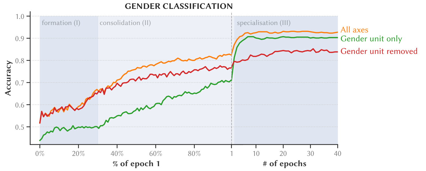
We first investigated how the LM learns to represent gender during training and how this representation becomes encoded in the input embeddings. To answer this question, we trained several linear classifiers to predict the gender of 82 gendered word pairs (e.g., "he"-"she", "son"-"daughter"). We analyzed snapshots at various points during training: after each epoch (one pass over all training data) and at multiple points during the first epoch. The LM was fully trained after 40 epochs.
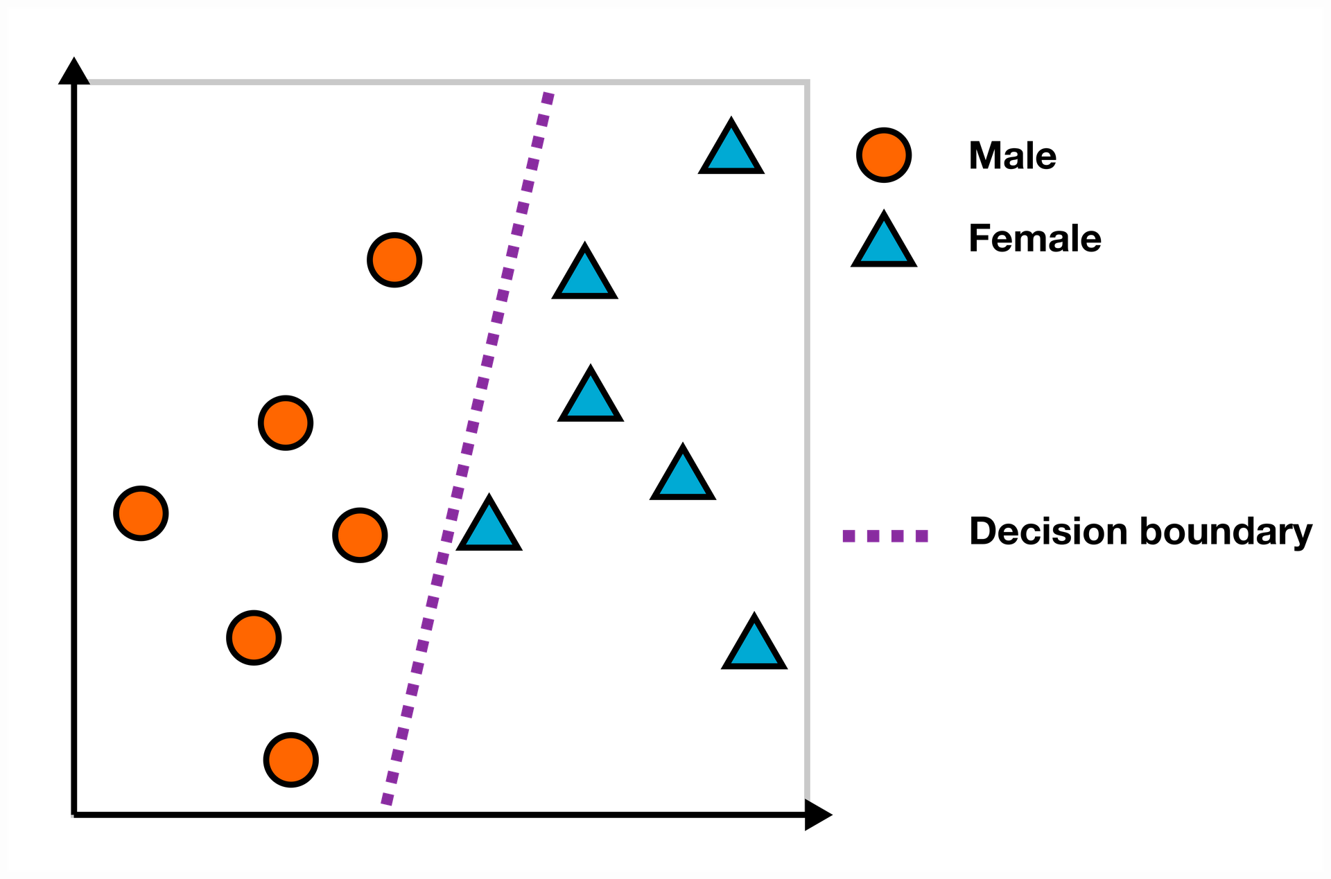
We tested these classifiers in two conditions: 1. Using all dimensions of the input embedding space 2. Using only the single most informative dimension (which we call the gender unit)
Interestingly, after just 2 epochs of training, using only the gender unit outperformed using all other dimensions of the input embedding space! This suggests that gender information becomes highly localized in the input embeddings early during training.
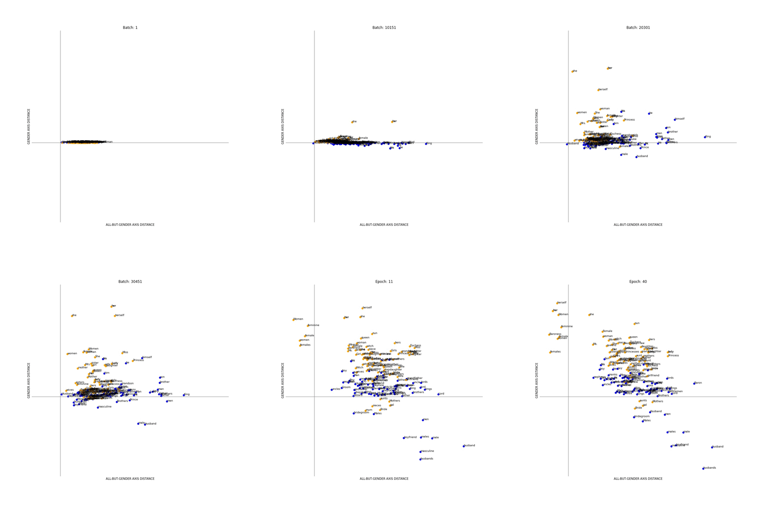
Another fascinating discovery was that the dominant gender unit appears to specialize in representing female words, while information about male words remains distributed across the rest of the embedding space. The animation below illustrates this phenomenon: - The top row shows correct predictions by the gender unit classifier - The right column shows correct predictions by the classifier trained on all other dimensions - Distance from the origin indicates how far a word is from the respective decision boundaries
Notice how words like "she", "her", "herself", and "feminine" quickly move to the top, while by the end of the animation, masculine words are only correctly predicted by the classifier that excludes the gender unit.
The Evolution of Gender Bias
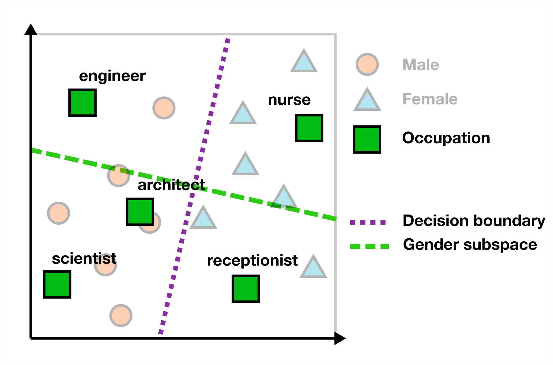
Using a linear decision boundary to study gender representation in embeddings aligns with one class of gender bias measures: those based on finding a linear gender subspace. Following Ravfogel, we define the gender subspace as the axis orthogonal to the decision boundary of a linear SVM trained to predict gender from a set of male and female words [10].
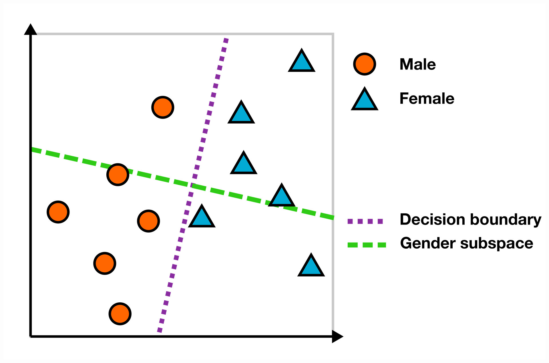
To determine a word's bias score in the embedding space, we measure its scalar projection onto the gender subspace. In the example below, words like "engineer" and "scientist" fall on the "male" side of the subspace (left of the purple decision boundary), while "nurse" and "receptionist" show female bias (right side). The further a word is from the decision boundary, the stronger its bias.
While this gives us a measure of gender bias in the LM's input embeddings, it's important to remember that this represents only one part of the model. The bias that actually affects users appears in downstream tasks, not in the hidden input embeddings. Unfortunately, the relationship between a model's internal bias and its downstream behavior isn't straightforward.
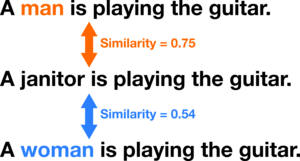
For this reason, we also measured gender bias in a downstream task – specifically, the Semantic Textual Similarity task for Bias (STS-B) [11]. In this task, the LM estimates the similarity between three sentences containing either "man," "woman," or an occupation term. The gender bias for that occupation is the difference in similarity scores averaged across 276 template sentences.
The example below shows how we calculated bias for "janitor" using one template sentence, resulting in a score of 0.75 - 0.54 = 0.21 (male bias).
Using these measurement tools, we tracked how gender bias in both input embeddings and the STS-B task evolved during training. We found significant gender bias in both representations (which correlated with actual gender distributions in US Labor Statistics [5]).
The figure below shows bias scores at three points during training. The bias measured in input embeddings reasonably predicted the bias in the STS-B task, although the correlation between these measures reached only 0.6 by the end of training – indicating important differences remain. One notable difference was a gender asymmetry in the input embedding bias (skewed toward female bias at epoch 40) that didn't appear in the downstream task.

Diagnostic Intervention: Changing Downstream Bias by Modifying Embeddings
While our findings showed correlation between input embedding bias and STS-B bias, we wanted to determine if there was a causal relationship. We conducted a diagnostic intervention to answer the question: Does debiasing the input embeddings measurably affect downstream bias?
Again following Ravfogel's method [10], we debiased the input embeddings by projecting all words onto the null-space of the gender subspace (the decision boundary), effectively removing gender information from this subspace. Since there may be multiple linear representations of gender, this procedure should be repeated several times. We indicate the number of debiasing iterations with k.
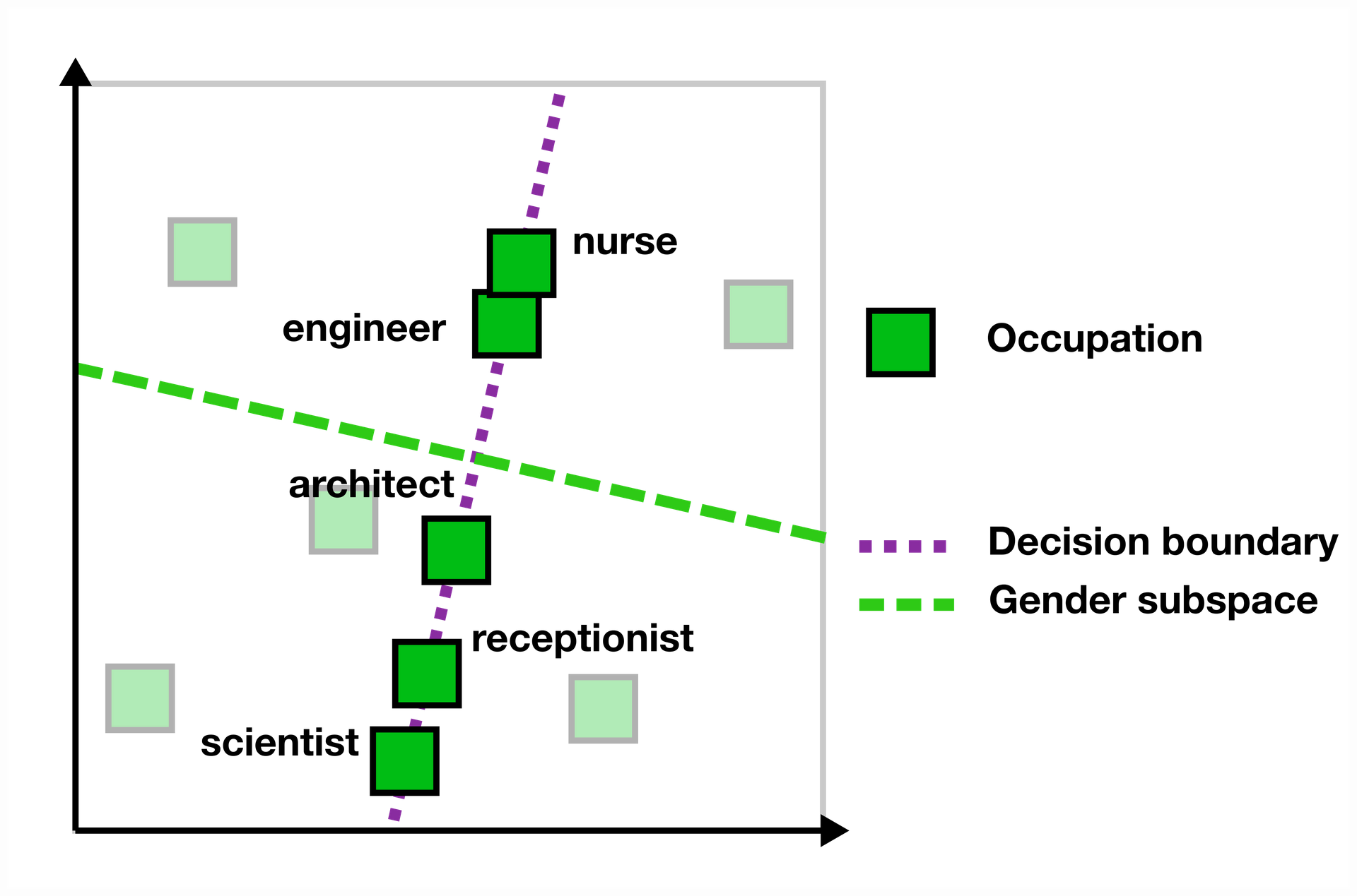
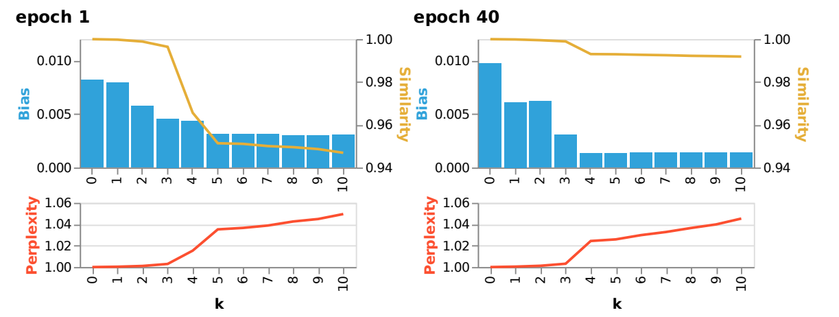
To study how debiasing input embeddings affects downstream STS-B task bias, we performed 10 debiasing iterations. For each step k, we measured: 1. The STS-B bias 2. The effect on the model's perplexity 3. The topological similarity of the embeddings compared to the original model
The figure below shows results for the LM after 1 and 40 epochs of training. We observed several surprising patterns:
-
While the original LM had higher bias at epoch 40, debiasing was much more effective at this later stage, ultimately resulting in lower bias. This aligns with our earlier finding that gender information becomes more localized over training, making it easier to remove selectively.
-
While extensive debiasing often damages the LM, applying just three debiasing iterations reduced bias without significant side effects. Both perplexity and embedding topological similarity remained close to pre-debiasing values.
Given the gender asymmetries we observed earlier, we also analyzed debiasing effects on female-biased and male-biased occupations separately. The figure below shows the impact on input embedding bias (left) and STS-B bias (right). Interestingly, a single debiasing iteration primarily reduced female bias in input embeddings (and even increased measured male bias) – possibly explained by the dominant gender unit's specialization in female word information.
Surprisingly, for STS-B bias, the first debiasing step reduced male bias more significantly. This discrepancy requires further research.

While we confirmed a causal relationship between input embedding bias and STS-B bias, more research is needed to understand their precise connection. It's particularly important to consider potential gender asymmetries in the model's internal representations, as naive mitigation strategies might introduce new biases through disparate effects on different social categories.
Conclusions
Our research revealed several key insights about gender bias in language models:
-
We identified distinct phases in the learning dynamics of gender representation and bias, characterized by changes in how locally gender information is represented and which dataset features explain these changes.
-
Gender becomes increasingly locally encoded in input embeddings during training, with the dominant gender unit specializing in representing feminine word information.
-
Bias in input embeddings reasonably predicts downstream bias. Debiasing input embeddings effectively reduces downstream bias, indicating a causal relationship.
-
We observed striking gender asymmetries, including the gender unit's specialization in female information and different debiasing effects depending on a word's gender bias. This underscores the importance of understanding how gender bias is represented within LMs, as naive debiasing approaches may inadvertently introduce new biases.
@article{van2022birth,
  title={The Birth of Bias: A case study on the evolution of gender bias in an English language model},
  author={van der Wal, Oskar and Jumelet, Jaap and Schulz, Katrin and Zuidema, Willem},
  journal={arXiv preprint arXiv:2207.10245},
  year={2022}
}